Tile coding for action-value functions.

Introduction

Tile coding is a technique used to represent multi-dimensional continuous spaces.

The space is covered by multiple overlapping tilings or grids. Tilings are offset from one another by a uniform amount in each dimension. Each tiling partition is a tile. A state is represented by the set of tiles it falls into across all tilings. This representation produces a sparse, binary feature vector, which is both memory-efficient and computationally efficient for moderate-dimensional problems.

Tile Coding Example

The figure below illustrates the concept:

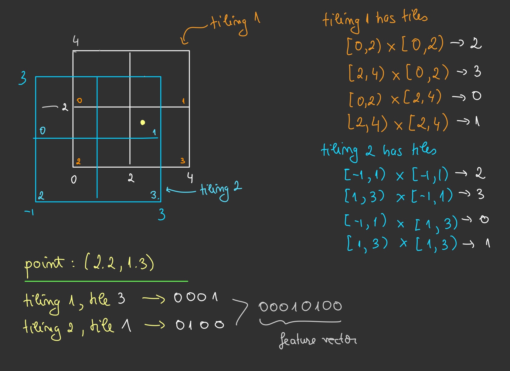
For practical implementations, see tilecoding and tile3.

Pros and Cons

Here are the main strengths and limitations of tile coding:

Advantages:

• Well-suited for linear function approximation.
• Simple to implement.
• Only a small number of features are active at any time, so computationally efficient.
• Compared to artificial neural networks, tile coding is more stable and less sensitive to hyperparameters.
• Because the features are indicator functions of overlapping tiles, the linear combination of them can approximate nonlinear functions of the raw state.

Disadvantages:

• The number of tiles grows with the number of state dimensions. For example, representing a humanoid robot with many degrees of freedom would require a very large number of tiles.
• Has a fixed representation of the state space. Once the tilings are set, the feature map is static.

Linear Function Approximation

Consider the state-value function \(V(s_t, \mathbf{w})\) with feature vector \(\boldsymbol{\phi}(s_t)\).
It can be represented as a linear combination of features, as follows

\[V(s_t, \mathbf{w}) = \mathbf{w}^\top \boldsymbol{\phi}(s_t), \quad \text{where} \quad \boldsymbol{\phi}(s_t) \in \{0, 1\}^n \quad \text{and} \quad \mathbf{w} \in \mathbb{R}^n.\]

For stochastic gradient descent (SGD), the update rule is

\[\mathbf{w}_{t+1} \leftarrow \mathbf{w}_t + \alpha(U_t - V(s_t, \mathbf{w}_t)) \boldsymbol{\phi}(s_t),\]

where \(U_t\) is the target value and \(\alpha\) is the step size.

For temporal-difference (TD) learning, the update becomes

\[\mathbf{w}_{t+1} \leftarrow \mathbf{w}_t + \alpha(R_{t+1} + \gamma \mathbf{w}^\top \boldsymbol{\phi}(s_{t+1}) - \mathbf{w}^\top \boldsymbol{\phi}(s_t)) \boldsymbol{\phi}(s_t),\]

where \(R_{t+1}\) is the reward at time \(t+1\), \(\gamma\) is the discount factor, and \(s_{t+1}\) is the next state.

SARSA with Tile Coding

Now consider SARSA, with an action-value function \(Q(s, a)\).
A natural choice of features is \(\boldsymbol{\phi}(s, a)\). Suppose we have discrete actions \(a \in \{1, 2, \ldots, K\}\).
The action-value function can then be expressed as

\[Q(s, a, \mathbf{w}) = \mathbf{w}_a^\top \boldsymbol{\phi}(s), \quad \text{where} \quad \mathbf{w}_a \in \mathbb{R}^n,\]

and the full weight matrix \(\mathbf{w}\) has shape \(K \times n\).

Since \(\boldsymbol{\phi}(s)\) is a binary vector (and thus sparse), the action-value function can be computed as

\[Q(s, a)=\sum_{i \in \text { active tiles }} \mathbf{w}_{a, i} \quad \text { for all } a=1, \ldots, K.\]

The greedy action is chosen as

\[a^*=\arg \max _{a \in\{1, \ldots, K\}} Q(s, a),\]

Note: Always break ties randomly to avoid bias.

Connections to Brain-inspired Approaches.

There’s actually a well-known connection between tile coding and how the brain may represent space. Here’s a link to a wikipedia page.

Conclusion

In summary, tile coding is a simple and efficient way to represent continuous spaces with sparse, binary feature vectors. However, this efficiency comes with limitations: the number of tiles increases with the dimensionality of the state space, which makes the method less practical for very high-dimensional problems.

References

[1] R. S. Sutton and A. G. Barto, “Reinforcement Learning: An Introduction,” MIT Press, 2018.